What is Azure Quantum? | Introduction to Quantum Computing

On February 1, Microsoft released Azure Quantum in “public preview”, making its cloud quantum computing platform available to everyone. But before I explain everything that Azure Quantum has to offer, I’m going to try to explain in a simple way what quantum computing is and why the scientific community has its hopes in it. If you already know what a qubit is, quantum entanglement and how a quantum algorithm works, you can skip the next section.

Introduction to Azure Quantum Computing

As you may know, classical computing uses a binary system of ones and zeros to represent information. We call each of these binary digits of information bits. Physically there are many ways to store these bits, for example, if electric current passes through a circuit we call it 1 and if not 0. The classic computers what they do is process this binary information through algorithms to solve problems.

Quantum computing takes advantage of the discoveries made by quantum physics at the atomic level to store information in tiny particles, such as ions. And it takes advantage of the strange and anti-intuitive quantum properties to process the information more quickly. By analogy to classical computing, the minimum unit of information in a quantum computer we call qubit.

What is a qubit?

Leaving aside the physical medium to construct a qubit, from a theoretical point of view we can say that a qubit, like a bit, can store two basic states that we will call |0〉 and |1〉. But in addition, it can contain a combination of the two states with a certain proportion.

What is superposition?

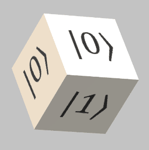
Qubit dice

Imagine that our qubit is some dice. If the dice has |0〉 on all its faces, throwing the die will always give the same result, |0〉. And the same if all faces are |1〉.

But if the die has |0〉 on three of its faces and |1〉 on the other three, when we roll the dice, we will have the same probability of getting |0〉 and |1〉. What will determine whether |0〉 or |1〉 comes out will be chance. These states in which chance determines the outcome of the launch based on the configuration of the dice, we call them superposition states.

Quantum computers allow operations on the qubits to change the number of faces that have |0〉 and |1〉 on our “dice”. The equivalence to the roll of the die would be the reading or measurement of qubits. When we measure a qubit, we can only get a |0〉 or a |1〉. Like when we roll the dice.

How is the state of a quantum computer stored?

To simplify it a lot, a quantum computer stores the probabilities of |0〉 and |1〉 of each qubit. For example, if we only have one qubit, the state of the computer could be as follows:

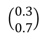
Where the first number, 0.3 (30%), indicates the probability that appears|0〉, and the second, 0.7 (70%), indicates the probability |1〉.

Another example, if in the qubit, we wanted to save a |0〉, the state would be  and if we wanted to save a |1〉 it would be  . This is the way to store the basic states.

Later we will see the exact way in which the state is saved, but for now think of probabilities facilitates the explanation.

Can we simulate a quantum computer on a classic computer?

With what we’ve seen so far, nothing would prevent us from building a quantum computer simulator by storing in our classic bits the probabilities of qubits. Basically, we’d need a couple of positive numbers for every qubit.

The problem is that when we have more than one qubit the state does not grow linearly, but exponentially. You’ll understand perfectly with an example:

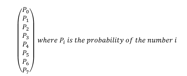
With a classic 3-bit computer we can store 8 numbers (from 0 to 7), that is 2³. But a quantum computer needs to store the probability of each of those 8 numbers, so the state would be:

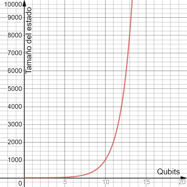
Ratio of qubits to state

Continuing with the die metaphor, imagine now that our quantum computer is a die that has 8 faces, and that we configure the die so that it has a number on each face, therefore, the probability of each number would be 0.125 (12.5%), meaning, P₀ = P₁ = … = P₇ = 0.125.

Therefore, to simulate a 100-qubit quantum computer we would need to store 2¹⁰⁰ numbers with the probabilities. To give us an idea, it is estimated that the amount of data used worldwide in 2021 is about 60 zettabytes (1 ZB = 10²¹ bytes = 1 trillion of GB). We would need more than 21 million “data worlds” to simulate just 100 qubits.

Actually, we don’t always need 2^N number to save the state of N bits. If the qubits are not entangled, we are good with 2 x N numbers. Storing the probabilities of each qubit separately, as if they were N independent quantum computers. Which brings us to the next question…

What is quantum entanglement?

Suppose a 2-qubit quantum computer. There are computer states that cannot be achieved by combining the independent states of the 2 qubits. When this happens, we say that these two qubits are entangled. The entanglement causes that the modification of one of the qubits affects also the other, and that the reading of one qubit conditions the reading of the other. By the way, you can perform entanglement of more than 2 qubits. Let’s see an example of entangled state between 2 qubits:

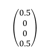
This state would be equivalent to a dice in which half of the faces have the number 0 (00 in binary) and in the other half the number 3 (11 in binary). It is impossible to get the same ratio of results with two independent dice that generate the 0s and 1s binaries separately. We would need two magic dice in order to achieve this, so that when throwing the second die always came out the same as in the first.

By the way, speaking of physics, it’s possible to take these two entangled qubits and physically separate them hundreds of miles from each other. Well, if we measure the first qubit and get a 0, we can assure 100% that when we measure the other qubit we will also get a 0. And the same with the 1. And this effect works instantly, surpassing the speed of light. The universe of quantum is not only random, but in a way, also magical.

The interference

Complex number in the plane

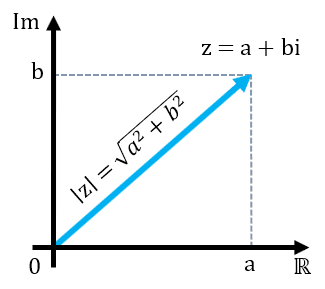
We only lack a concept to be able to understand how quantum algorithms work, the interference. With what we’ve seen so far, we could have a quantum computer with a brutal capability, but it would be very difficult to use it to solve problems. The grace of quantum computers is that the numbers stored in the state are not positive numbers, but complex numbers. So instead of directly storing the probability, it stores what we call amplitudes.

To know the probability, we just have to calculate the amplitude module and square it up. Geometrically, it is equivalent to the square of the distance between a point in the plane and the origin of coordinates. Of course, you have to keep fulfilling that the sum of all probabilities is 1.

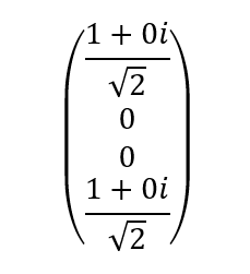
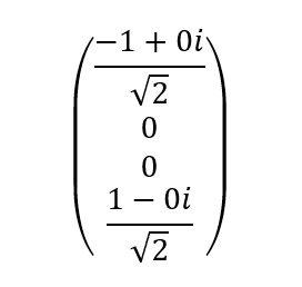
For example, the entangled state we saw in the previous section would actually be stored like this:

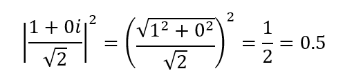
To calculate the probabilities, we would have to take each amplitude and do the following:

For example:

The advantage of storing amplitudes is that we can play with negative numbers, both in the real part and in the imaginary part of complex numbers. For example, the next state is fully equivalent to the previous one in terms of the resulting probability:

With interference what we do is we make transformations in the state so that the amplitudes of the incorrect solutions to the problem are subtracted and tend to zero and the amplitudes of the correct solutions are added and amplified so that the probability of obtaining such solutions are as high as possible.

The name interference comes from the wave field. Think of each amplitude as a wave. If we add two waves in which the ridges and the valleys coincide, the wave is amplified, but if we do just the opposite the waves cancel out. This is what is called constructive and destructive interference, respectively.

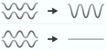
Wave interference

How do quantum algorithms work?

Most quantum algorithms fit the following scheme:

• Preparation phase: An input qubits preparation is performed in which the initial values of the qubits are set. Usually, part of this preparation is to put the qubits in superposition. This is what allows us to take advantage of quantum parallelism to gain speed.
• Calculation phase: transformations are made on the qubits trying to amplify the expected results and minimize the incorrect results, taking advantage of quantum interference. To achieve this, it is usually necessary to entangle qubits.
• Measurement phase: Measure qubits, thus destroying the internal state of the measured qubit amplitudes and obtaining a classic output of 1s and 0s.
• Iterative phase: as the result obtained is probabilistic, the expected result is not always obtained, so it is usually necessary to check if the result obtained is valid or it is necessary to run the algorithm again. Other times, you simply have to iterate many times to get the result statistically.

Complexity of quantum computing

At this point you may be wondering, why do quantum computers work in this complicated way? Is this whole mess of complex numbers, amplitudes and so on necessary?

The answer is quite simple: nature works like this. What scientists have done has been to find a mathematical model that fits like a glove to quantum mechanics. And in this way take advantage of the operation of nature to make calculations that would be impossible to carry out in the classic computers.

Quantum algorithms developed so far have already demonstrated their superiority over classical homologous algorithms for reduced problem sizes. Therefore, if you can build a quantum computer with enough qubits, you can solve problems with sizes so far unapproachable.

Perhaps the most famous algorithm is that of Shor, which allows to perform the factorization of the public key in its prime factors, pulling down current encryption systems with public key that are used for example for Internet communications. Such factoring would cost thousands of years to do on the most powerful classical computer, while on a quantum one it could be done in hours.

What is Azure Quantum?

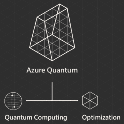
Azure Quantum

Azure Quantum is a service offered by Microsoft through its cloud, Azure. This service has two distinct parts, quantum computing and optimization. Both can be deployed by creating a Quantum Workspace resource in Azure.

Quantum computing

With Quantum computing from Azure, we can develop quantum algorithms using the Q# programming language and the QDK (Quantum Development Kit). Both Q# and QDK are open source. QDK includes specific libraries for chemistry, machine learning and qubit calculations. And we can use our favorite tools: Visual Studio, VS Code and Jupyter Notebooks.

The algorithms we implement can be executed on a small scale using the local QDK simulator, and we can also upload them to the cloud in the form of jobs, using a Quantum Workspace.

At the time of uploading a job we can choose which supplier we want to run it in. Microsoft puts at our disposal different suppliers that offer us simulators of quantum computers of greater capacity than our local and also real quantum computers with a few qubits.

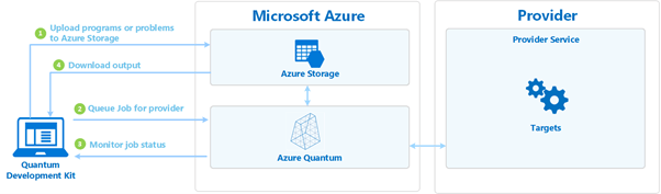
Running algorithms in Azure Quantum

Currently, we have available two real quantum computer providers implemented by ion traps:

• Honeywell Quantum Solutions:
  • System Model H0: 6 qubits
  • System Model H1: 10 qubits
• IonQ:
  • Trapped Ion QC: 11 qubits

In the future, more suppliers will be added, such as the superconductor-based quantum computer from Quantum Circuits Inc.

Be careful when comparing the power of quantum computers by the number of qubits because it can be misleading. The measure to take into account is quantum volume. For example, the H1 de Honeywell model has a quantum volume of 128, the largest in the world since November 2020. Although perhaps for a short time, because IonQ has assured that in 2021 will offer through Azure Quantum a computer with 32 qubits and a quantum volume of nothing more and nothing less than 4 million!

By the way, a great advantage of ion trap-based computers is that thanks to the mobility of the ions you can perform the quantum entanglement between all the qubits you want.

However, thanks to Azure Quantum and Q# we can abstract from the hardware that will run our algorithm. However, it should be noted that the design of the algorithm can affect performance depending on the hardware used.

Optimization

With Azure Quantum Optimization, we have access to optimization algorithms made by Microsoft and other vendors. Optimization problems are solved by searching through the possible solutions. The best solution is the one with the lowest cost, although it is not always possible to find the best solution. A typical problem of optimization is the problem of the traveller (Travelling Salesman Problem), who tries to find the shortest route to travel through a set of cities and return to his home.

In order to use these algorithms, we must be able to define the problem to be solved in the terms of specification defined by the solvers. For this we will use the Python SDK: azure-quantum. These algorithms will run on classic hardware in Azure.

Currently, we have two optimization algorithm providers available, with the following solvers:

• Microsoft QIO (Quantum-Inspired Optimization):
  • Simulated annealing
  • Simulated annealing (Parameter-free)
  • Parallel tempering
  • Parallel tempering (Parameter-free)
  • Quantum Monte Carlo
• 1Qloud Optimization Platform:
  • Tabu Search Solver
  • Path-Relinking Solver
  • PTICM Solver

The advantage of using these algorithms inspired by quantum computing is that we can use them in real problems with improved speed, without having to wait for the evolution of quantum computers. And when the long-awaited quantum supremacy comes, we won’t have to change anything to take advantage of the new computing power.

Summary and conclusions

We’ve taken a brief tour of some of the most important concepts in quantum computing:

• Qubit as quantum bit.
• Superposition to allow intermediate states of the qubit between 0 and 1.
• The state of the quantum computer as a vector of size 2^{nº of qubits}.
• The extraordinary properties of quantum entanglement to coordinate two or more qubits.
• The use of quantum interference to amplify valid solutions to a problem and decrease invalids.
• The general scheme of quantum algorithms, combining all the above.

We have also seen how Microsoft, through Azure Quantum, provides us with the necessary tools to develop quantum algorithms both in simulators and in real quantum computers of a few qubits. In addition, it offers us some algorithms already implemented that we could use to solve optimization problems.

No wonder the expectations placed on the future of quantum computing are so high. Given the potential computing power of a quantum computer with a few hundred qubits and the speed at which quantum volume is increasing, the future is certainly encouraging. Not in vain, companies and governments around the world are investing millions in quantum technology research. For example, the European Union, with its large-scale initiative called Quantum Flagship, will invest €1 billion over 10 years.

But there are also important challenges ahead of the long-awaited quantum advantage. This is the case of the feared quantum decoherence that must be avoided during the execution of the algorithms since it decomposes the superposition and entanglement of the qubits.

In any case, we are grateful for the continuous advance of the development tools for quantum computers that will guarantee us a mature development environment for the next quantum revolution.